R language

What? And why?

R is a language developed in an open-source environment. It is an interpreted language that does not need to be compiled by a compiler, and allows rapid programming with its interactive command-line interface (similar to the Python one) and scripting.

Due to its straightforwardness, it is widely used in data mining and data analysis. As one of the most commonly used numerical computing programming languages, it is worth having a brief introduction to it.

RStudio

We hardly ever just write code from the command line, and even less if the language we are using is mainly to get visual analysis of the data. Therefore, the most common way to use R is by Rstudio, a Graphical User Interface software to develop R code.

rstudio_logo

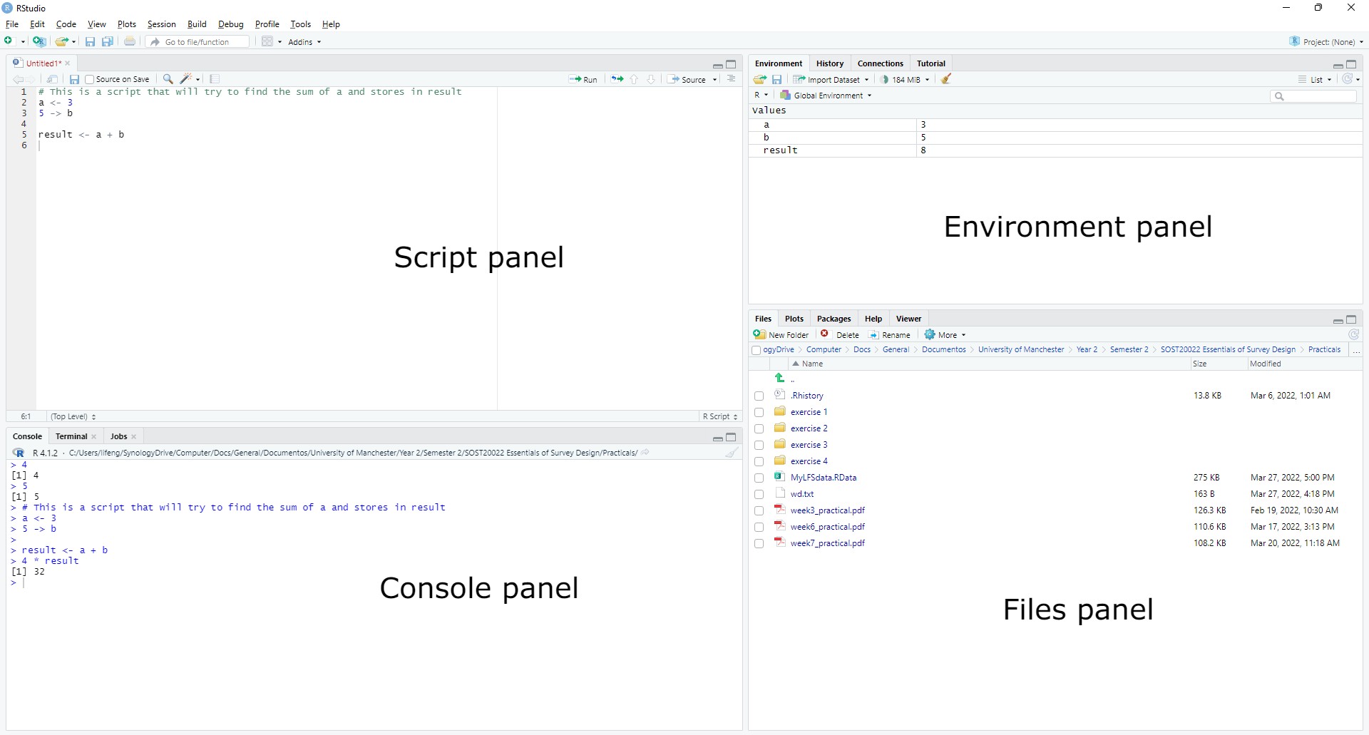
Once downloaded and inside, 4 panels (3 if the script panel is not opened) will show up. From left top to right bottom, they are:

Script panel: where you can write blocks of code to be executed. A very helpful functionality that I find, is that it allows you to select the lines of codes that you want to run if not all, by selecting them and pressing run.
Console panel: where the interactive terminal is. You can either enter code here to be executed or use a script. The outputs e.g. print outputs will be shown here.
Environment panel: where you can see all the variables stored currently.
- Another useful tab in this panel is history, where you can check all previously executed commands.
Files panel: where you can see the files in a explorer format.
- Plots tab allows you to visualise output of any R figures.
- Packages to explore any installed R packages.
- Help outputs the relevant information when help(“some_command”) is called

rstudio_4_panels

R packages

R as a community comes with the huge support of packages. Install a package with

1	install.packages("package_name")

Incorporate packages into your library with

1	library("package_name")

These actions can also be done in the RStudio GUI.

R scripts

Very often, we need to use a piece of code on multiple occasions, that’s why it is useful to store them in a file. These files are called R scripts.

# This is a script that calculates the root mean square of two numbers

a <- 1 # <- is the assignment operator
b <- 2

rms <- sqrt(a^2 + b^2) # ^ is the exponent operator, sqrt is the square root function

print(rms)

Loading data

R‘s default reading function is read.table, and is a bit limited in the way that it can only read human-readable data files (e.g. tab-separated, comma separated). The result is a data.frame object.

1	data <- read.table(filename, header=TRUE, sep="\t")

Data structures

Vector

Vector is a group of values ordered as an array in which all elements should be of the same type.

There are several ways of instantiating a vector:

1
2
3

v <- c(1, 2, 3, 4, 5)
v <- 1:3 # [1, 2, 3]
v <- c("apple", "banana", "cherry") # a character vector

To extract from a vector

1
2
3

v[1] # first element
v[1:3] # first three elements (vector)
v[c(1, 3, 5)] # first, third and fifth elements, notice 1-indexed

List

List is a vector that allows multiple types of values.

List follows the same creation and extraction rules as a vector, only that each element is also considered as a list. Hence:

l <- list(1, "a", TRUE, c(-1, -2, -3))

l[[2]] # second element, "a"
l[[4]][3] # third element of the fourth element, -3. Do not use l[[4, 3]]

Matrix

Matrix is a vector of vectors; a 2D vector, and has a rectangular shape.

Create a matrix

m <- matrix(c(1, 2, 3, 4, 5, 6), nrow=2)
     [,1] [,2] [,3]
[1,]    1    3    5
[2,]    2    4    6

n <- cbind(c(8, 6, 2), c(1, 2, 3), c(2, 3, 3)) # cbind joins the vectors into a matrix
     [,1] [,2] [,3]
[1,]    8    1    2
[2,]    6    2    3
[3,]    2    3    3

Extract an element or a vector from a matrix

1
2
3

m[1, 2] # first row, second column; 3
n[1, ] # first row; [8, 1, 2]
n[, 3] # first column; [2, 3, 3]

Data frame

Data frame is the most commonly used data structure in R. It is a matrix in which each column is considered an attribute of the data, and each row is considered an observation. As attributes, columns always have their name. If not declared explicitly, they will be called X1, X2, X3, etc.
For instance, in a survey, each row is a person, and each column is a variable from a question (e.g. age, sex, income).

The read.table automatically loads data into a data frame. Other way of creating one is from a matrix.

df <- data.frame(m)
  X1 X2 X3
1  8  1  2
2  6  2  3
3  2  3  3

The extraction follows the same rules as for matrices. One difference is in the extraction of columns with df[, 2] and df[2]. Notice as we have a name for each of the columns, we can extract the column with the name.

df[, 2] # if with 2 coordinate system, the result is flattened
1 2 3

df[names(df) == "X2"] # extract column X2
df[2] # same effect, second COLUMN, not ROW
  X2
1  1
2  2
3  3

You may have guessed, names in column is fairly important, here is how to change them:

names(df) <- c("new_name_1", "new_name_2", "new_name_3") # change all names

names(df)[1] <- "new_name_1" # change only the first name
names(df)[names(df) == "X1"] <- "new_name_1" # change column named X1

Boolean and masks

Data structures can interact with boolean values, providing filter functions (mask).

# runif(n) creates n random numbers between 0 and 1
m <- cbind(runif(10), runif(10), runif(10))

        [,1]      [,2]       [,3]
[1,] 0.16911856 0.8984747 0.10109347
[2,] 0.19173547 0.9902025 0.67376471
[3,] 0.89473736 0.3980775 0.96819965
[4,] 0.95936313 0.9812951 0.26555639
[5,] 0.31889684 0.5200781 0.35668182
[6,] 0.54475071 0.6374638 0.64514961
[7,] 0.10041832 0.1779460 0.05627609
[8,] 0.07695519 0.9616795 0.26788061
[9,] 0.88356189 0.6104990 0.10228830
[10,] 0.07814162 0.8857073 0.42943937

# boolean mask for all values greater than 0.5
m > 0.5 
    [,1]  [,2]  [,3]
[1,] FALSE  TRUE FALSE
[2,] FALSE  TRUE  TRUE
[3,]  TRUE FALSE  TRUE
[4,]  TRUE  TRUE FALSE
[5,] FALSE  TRUE FALSE
[6,]  TRUE  TRUE  TRUE
[7,] FALSE FALSE FALSE
[8,] FALSE  TRUE FALSE
[9,]  TRUE  TRUE FALSE
[10,] FALSE  TRUE FALSE

# applicable to sub-matrix
m[2, ] > 0.5 
[1] FALSE  TRUE  TRUE

# some common processing is achieved with masks, such as setting all values between 0.5 and 0.8 to 1. Operator and (&), or (|), and not (!)
m[m > 0.5 & m < 0.8] <- 1
        [,1]      [,2]       [,3]
[1,] 0.16911856 0.8984747 0.10109347
[2,] 0.19173547 0.9902025 1.00000000
[3,] 0.89473736 0.3980775 0.96819965
[4,] 0.95936313 0.9812951 0.26555639
[5,] 0.31889684 1.0000000 0.35668182
[6,] 1.00000000 1.0000000 1.00000000
[7,] 0.10041832 0.1779460 0.05627609
[8,] 0.07695519 0.9616795 0.26788061
[9,] 0.88356189 1.0000000 0.10228830
[10,] 0.07814162 0.8857073 0.42943937

Other common syntax

R has a very straightforward syntax, some of its regular syntax example are the following.

Loops

for (i in 1:10) {
  print(i)
}

while (i < 10) {
  print(i)
  i <- i + 1
}

Conditionals

if (i > 5) {
  print(i)
} else {
  print(i + 1)
}

Functions

1
2
3

plus_one(x) {
  x + 1
}

Visualisation packages

A good place to start is the ggplot2 package.

R Markdown

R Markdown is a simple syntax for writing R code in a Markdown-like format.

Conclusion

R is a very powerful language, and it is very easy to learn. This has been a quick introductory post about its general syntax and some of the most common features. The next R tutorial may be a real example of how to use it to extract wanted data and perform statistical analysis on it.

Introduction to R

R is a numerical computing language commonly used and compared to Matlab, Python, etc. Most importantly, it is the language that I use for statistical analysis in a survey course. Hence, this little introduction to the R language.