Project Chronicles: Game of Life

Conway’s Game of Life

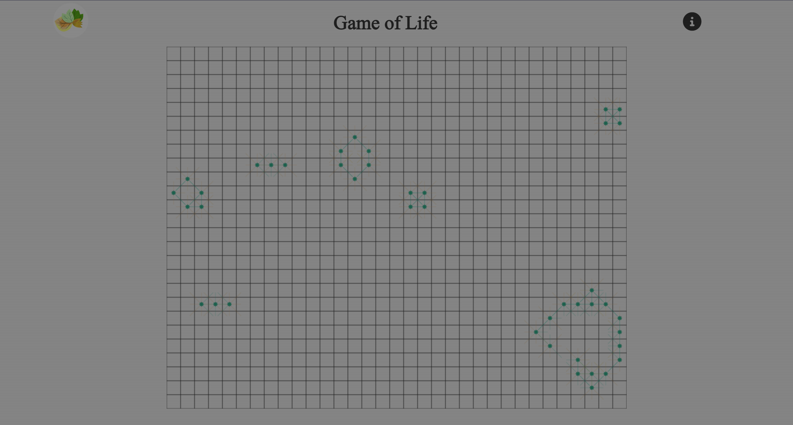
Conway’s Game of Life is a cellular automaton. Although it is called a “game”, it is a zero-player game. In this automaton, cells reproduce, evolve, and destroy themselves. They either form ordered tribes and “civilizations”, or silently vanish in history. I drew a dynamic, visual game of life through simple HTML, CSS and JS. We play the role of “the highest”, either indifferently observing the evolution of life, or altering the life and death of a cell with a single click to control the rise and fall of civilizations. For more information about this project, please go to Introduction , and to Project itself.

Project Epiphanies

Through the development of the project, there were some hard challenges from the project that I learnt a lot, which I also think are useful for future reference. The hits from this project are:

• Analysing CSS clamp for different situations
• Take a drawn pattern on a JS canvas, duplicate it and rotate it to a different angle.

CSS clamp

clamp syntax

I’m sure you’re quite familiar with the clamp syntax, but in case you need to, check the documentation if necessary.

clamp variables

CSS’s clamp function accepts the following variables:

clamp(MIN, VAL, MAX)

and then returns a value that depends on these three variables. In between, if VAL corresponds to a value that is not less than MIN and not greater than MAX, then clamp will return VAL.

In this description, you can see that MIN and MAX play the roles of maximum and minimum values. If VAL is less than MIN then MIN is used. Similarly, if VAL is greater than MAX then MAX is used.

This function can be implemented actually by earlier functions with MAX(), min(), what’s more, a clamp is exactly equivalent to:

max(MIN, min(VAL, MAX))

Clamp doesn’t only combine them, but optimizes the counter-intuitive problem that the names max() and min() bring. For example, when we want to set a minimum unit of font size, min() is probably the first thing that comes to mind. But this will only further reduce the font size. What we need is max() to choose the smallest font size when there is a smaller one. Clamp solves this counter-intuitive problem nicely.

clamp example

font-size: clamp(5rem, 10vw, 20rem)

clamp analysis

Readers may have a doubt while reading, with VAL and MIN (with MIN as an example but MAX also applies) as fixed CSS values, how can they be VAL larger than MIN from time to time and VAL smaller than MIN in other times?
The answer is simple: when the value depends on the size of other elements and is dynamically adjusted, then the values are not fixed any more.

For example, in the last clamp code example, 10vw is 200px when the screen size is 2000px wide. Suppose at this point 1rem is equivalent to 16px, then MIN is equal to 80px. It is easy to see that at this point clamp will return 200px (no 320px greater than 20rem).

However, if the user is reading on the phone screen, then the screen size may be reduced to 400px width. At this point, 10vw is equal to 40px, while 5rem is still equal to 80px (in the real case, the cell phone’s rem will be smaller). Then, according to the rules of clamp, at this time VAL < MIN, so it will return the 80px of MIN, complying with the minimum font size.

So it can be seen that CLAMP can conveniently limit the size to achieve a dynamic limiting effect. However, it can not only balance between too large and too small but also extend the values more extreme beyond the proportion.

Two combinations of clamp

Up to now, I don’t know if you have noticed, but the variables of the clamp example I gave are of this form:

clamp(fixed, scale, fixed)

What if we take this form:

clamp(scale, fixed, scale)

What happens if you use this clamp? For this reason, I will call the two different forms of clamps by their effects as stable clamps and dynamic clamps respectively.

Stable clamp

Stable clamp is how we normally use clamp, for example, to stabilize font size, image size, etc.

clamp(fixed, scale, fixed)

Due to the fixed value limit, this value does not usually change drastically depending on the size of the parent element/screen. For example, it will not become too small for a small phone screen, or too large for a large computer screen. This is why stable clamps are very suitable for important elements that need to be stable, such as fonts, images.

Dynamic clamp

Dynamic clamp is required for fewer scenarios, examples include margin, padding and border.

clamp(fixed, scale, fixed)

In the case of preferably fixed values, it means that the size of this element will be maintained even under different screens. In this sense, this clamp applies to elements that need to be fixed in size, such as images sometimes. But in most cases, we can take full advantage of the scale size limited by both ends, and the preferred fixed value simply acts as a trigger line to split the proportion needed for larger screens and the proportion needed for smaller screens.

The advent of stable clamps has solved the problem of making the size of the two ends converge to a balanced middle value. So the meaning of dynamic clamps will be the opposite, that is, increasing the difference between the two ends. This means that on small screens the element will become smaller than the anchored scale size, and on large screens, it will be larger than the anchored scale size. So variation clamp is suitable for less important, secondary elements, elements that leave space for more important elements when the screen is small; and elements that can fill in the gaps when the screen is large, such as margin, padding and border.

Short summary

CSS clamp is a quite useful function, which can be dynamically adjusted to different needs. If you want to study the most correct values of clamp, you need a mix of scale and fixed variables to achieve the best performance. For specific values, please refer to the search article on the web for the keywords related to the perfect variables to fit a clamp.

JS canvas pattern flipping

For the presentation of the Game of Life selection, I used HTML canvas and JS to render dynamic visualization. So I drew the cells using the built-in drawing function from canvas context. So how should each life be represented? In the end, I decided to use a lap of leaves to represent the cells after a few minutes of thinking. Resulting figure: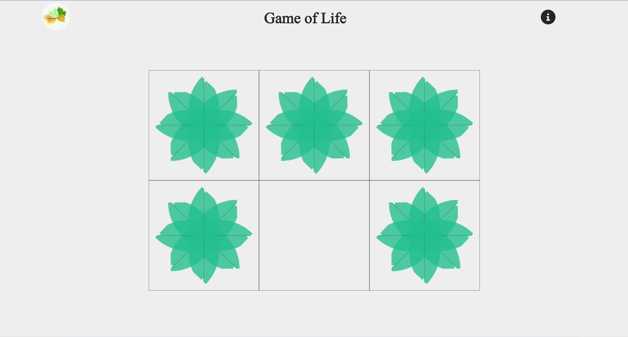

How to implement it exactly? The function drawCell() that draws a whole cell looks like this:

// Draw whole cell
drawCell = (color, size) => {

    // Localise center of the diagram
    // i and j are attributes of each cell from Cell class
    // grid_size is the length of the square sides that each cell is in
    const x_center = (this.i + 0.5) * grid_size;
    const y_center = (this.j + 0.5) * grid_size;

    // ...

    // Draw each leaf
    this.drawLeaf(Math.PI / 4, x_center, y_center, size, color);

    // As many directions as wanted, towards different angle
    this.drawLeaf(Math.PI * 3 / 4, x_center, y_center, size, color);
    this.drawLeaf(Math.PI * 5 / 4, x_center, y_center, size, color);
    this.drawLeaf(Math.PI * 7 / 4, x_center, y_center, size, color);

    this.drawLeaf(0, x_center, y_center, size, color);
    this.drawLeaf(Math.PI/2, x_center, y_center, size, color);
    this.drawLeaf(Math.PI, x_center, y_center, size, color);
    this.drawLeaf(Math.PI*3/2, x_center, y_center, size, color);
}

We first need to draw one leaf, which is a base unit. Then we can call this leaf function and rotate it to different angles.

Draw a leaf

In the drawCell() function, drawLeaf() is called several times to form a cell pattern with multiple leaves clustered around it. And drawLeaf() looks like this.

// Draw single leaf
drawLeaf = (deg, x_center, y_center, size, color) => {

        // Draw 1 leave
        let p1 = {x: x_center, y: y_center - 1/2*size};
        let c1 = {x: x_center + 1 / 3 * size, y: y_center - 1 / 6 * size};
        let p2 = {x: x_center - 1 / 6 * size, y: y_center - 1 / 6 * size};
        let c2 = {x: x_center + 1 / 3 * size, y: y_center - 1 / 6 * size};
        let p3 = {x: x_center - 1/9 * size, y: y_center};
        let p4 = {x: x_center + 1/16 * size, y: y_center};
        let c4 = {x: x_center - 1/3 * size, y: y_center - 1/6 * size};
        let p5 = {x: x_center, y: y_center - 1/3 * size};
        let c5 = {x: x_center + 1/12 * size, y: y_center - 5/12 * size};

        ctx.beginPath();
        ctx.moveTo(p1.x, p1.y);
        this.drawCurve(p1, p2, c1, 1 / 2 * size);
        this.drawCurve(p2, p3, c2, 1 / 2 * size);
        ctx.lineTo(p4.x, p4.y);
        this.drawCurve(p4, p5, c4, 1 / 2 * size);
        this.drawCurve(p1, p5, c5, 1 / 12 * size);
        ctx.fillStyle = color;
        ctx.fill();

        // Draw the stems
        ctx.beginPath()
        ctx.moveTo(p1.x, p1.y);
        ctx.lineTo(x_center, y_center);
        ctx.strokeStyle = this.alive ? colors.vein_alive : (this.next_gen < 3 ? colors.vein_under_population : colors.vein_over_population);
        ctx.stroke();
        ctx.closePath();
    }

The result looks like this.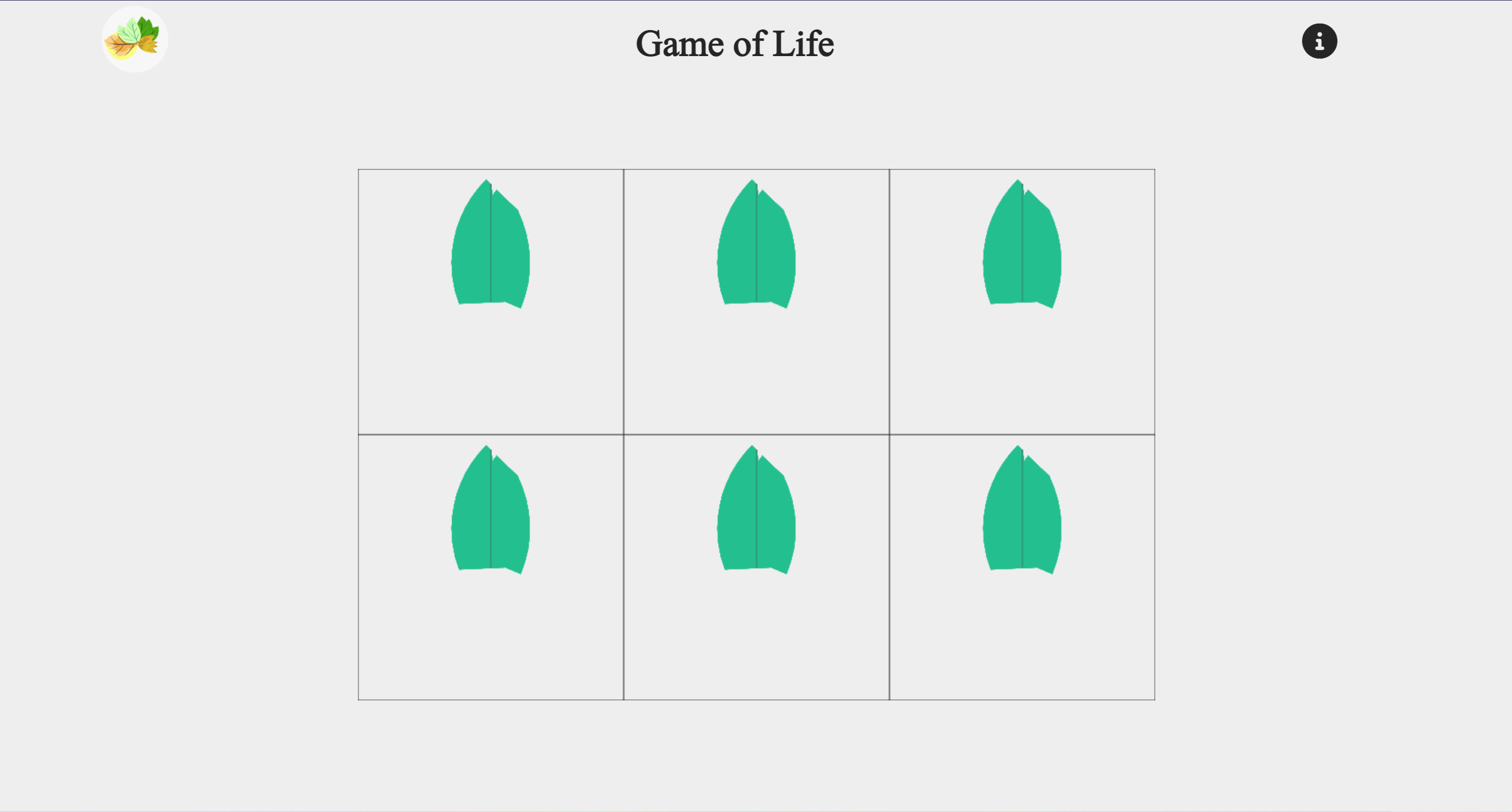

This example, if run, will only work for one leaf, and later we will see how to copy and rotate it. For now, let’s briefly see how to construct one leaf.

Point, Line, Surface

This method that I use is rather clumsy. It might be better to use the drawn picture directly and then have the canvas draw it for you.

The steps in between are not too difficult in order to draw this leaf. First, assuming that we are drawing the leaf pointing upwards, the first step is to figure out each of the key points used to outline it. What is a key point? It refers to the points of change when drawing the contour lines. For example, if we want to draw the sides of a square, then its four corners are the key points because the line will change at this point. Similarly, this applies to arcs, where the intersection of two different arcs is a key point. In this example, p1 to p2 depicts the upper left arc, while p2 to p3 outlines another arc with different circle centers c1 and c2 (p.s. they are the same now, but the previous pattern version had two different circle centers, and it’s more intuitive to split it into two parts, so I kept both circle centers).

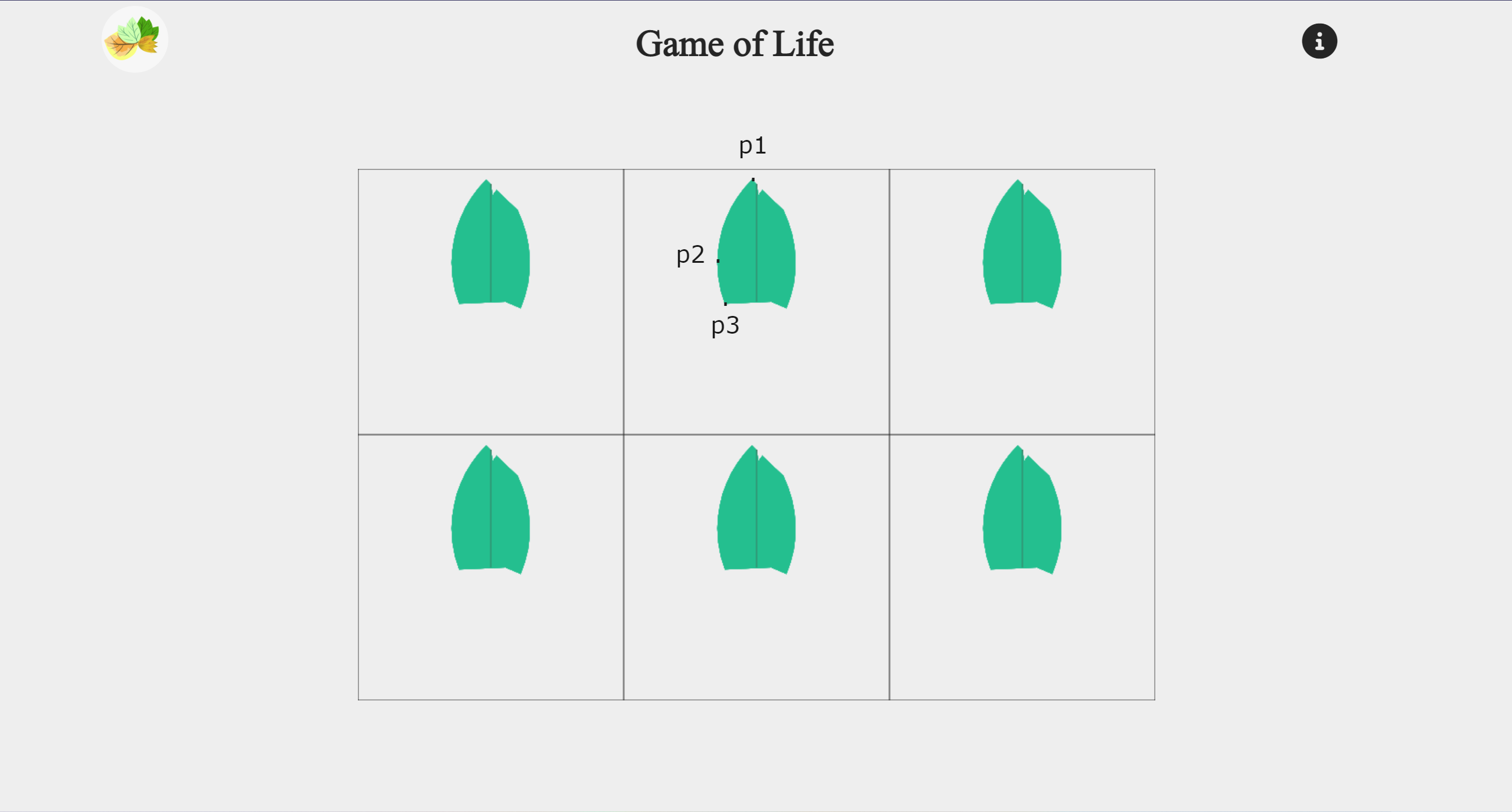
Regarding the coordinate system of the key points, I used the center point of the respective X and Y axes as the origin (0, 0) coordinate in each cell. The top is +y, the bottom is -y, the left is -x, and the right is +x. This is useful when copying and rotating other leaves according to the center point, after all, the axis/point of rotation is the center point of X and Y axes. Of course, you can also use the upper left corner as the origin of the coordinate system. Then, find the relative coordinates of each key point with their respective centroids, notice that it is a rather lengthy step full of trials.

After using this method, you can then connect the points into a set of line segments. For example, drawCurve() is a custom function of the Cell class, but inside it is actually a ctx.arc(), a built-in function for drawing curves. There is also, for example, lineTo() function for drawing lines, which draws a basic straight line.

The last thing is to fill the area connected by the lines into one face of the complete leaf. The filling can be done using ctx.fill(). In the end, I have also added some lines to pretend leaf veins, as an embellishment.

Draw multiple leaves

It’s not hard to copy and paste to draw multiple leaves, you just need to call drawLeaf() a few more times. The question is how to rotate them regularly?

For this kind of method that requires angle and periodicity, the first thing that usually comes to my mind are the trigonometric functions. If sin and cos are used properly to add, subtract, times 0, times 1, then is it possible to achieve this effect? The answer is yes.

At first, I thought this approach: assume that each point has x and y offsets, called dx and dy, which can be positive or negative or none. This offset d is the difference with the origin, for example, the dy of p1 is -1/2. Ignore size for now because its value is constant. Then you can use cos and sin to periodically increase and decrease d. For example, the p1-dx of the upper leaf is +dy on the right-pointing leaf, and this mental picture should not be hard to imagine, so you readers can try it.

Naive attempt

The dx and dy of each point change for each angle, even to the point where dx is attached to y and dy is attached to x. This process is periodic, which ensures that the coordinates of the leaves are cyclic. Of course, when dx and dy are no longer necessarily the offsets that represent x and y at different angles, then we give them a different name. We call the x offset of the original leaf d1 instead of dx and the y offset d2 instead of dy.

This periodicity and offset may sound roundabout; a tabular representation would be:

90º leaf	xd1	xd2	yd1	yd2
Scale	1	0	0	1

This should not be difficult to understand. In the most primitive 90° leaf, how much d1 and how much d2 does x have? Because we have already defined the x offset of the primitive leaf as d1 and the y offset is d2, so x has full d1 and no d2; while y has full d2 and no d1.

Later, I took this for granted that the rest of the angle should follow the same rules.

Any leaf	xd1	xd2	yd1	yd2
Degrees	sin	cos	cos	sin

This gives us the following code:

// Attempt for multiple leaves
drawLeaf = (deg, x_center, y_center, size, color) => {
    let cos = Math.cos(deg);
    let sin = Math.sin(deg);

    // Draw 1 leave
    // let p1 = {x: x_center, y: y_center - 1/2*size};
    // let c1 = {x: x_center + 1 / 3 * size, y: y_center - 1 / 6 * size};
    // let p2 = {x: x_center - 1 / 6 * size, y: y_center - 1 / 6 * size};
    // let c2 = {x: x_center + 1 / 3 * size, y: y_center - 1 / 6 * size};
    // let p3 = {x: x_center - 1/9 * size, y: y_center};
    // let p4 = {x: x_center + 1/16 * size, y: y_center};
    // let c4 = {x: x_center - 1/3 * size, y: y_center - 1/6 * size};
    // let p5 = {x: x_center, y: y_center - 1/3 * size};
    // let c5 = {x: x_center + 1/12 * size, y: y_center - 5/12 * size};


    // Draw leaf depending on degrees
    let p1 = { x: x_center - sin * 1 / 2 * size, y: y_center - cos * 1 / 2 * size };
    let c1 = { x: x_center + cos * 1 / 3 * size - sin * 1 / 6 * size, y: y_center + sin * 1 / 3 * size - cos * 1 / 6 * size };
    let p2 = { x: x_center - 1 / 6 * size, y: y_center - 1 / 6 * size };
    let c2 = { x: x_center + cos * 1 / 3 * size - sin * 1 / 6 * size, y: y_center + sin * 1 / 3 * size - cos * 1 / 6 * size };
    let p3 = { x: x_center - cos * 1 / 9 * size, y: y_center - sin * 1 / 9 * size };
    let p4 = { x: x_center + cos * 1 / 16 * size, y: y_center + sin * 1 / 16 * size };
    let c4 = { x: x_center - cos * 1 / 3 * size - sin * 1 / 6 * size, y: y_center - sin * 1 / 3 * size - cos * 1 / 6 * size };
    let p5 = { x: x_center - sin * 1 / 3 * size, y: y_center - cos * 1 / 3 * size };
    let c5 = { x: x_center + cos * 1 / 12 * size - sin * 5 / 12 * size, y: y_center + sin * 1 / 12 * size - cos * 5 / 12 * size };

    // ...

BUT, once you try to draw with this function, there will be an error, the leaves simply do not look like leaves and coordinates look disordered. To be honest, my heart broke when the leaves didn’t show up correctly even though I spend so much time analysing them. I obviously couldn’t give up at this point, so I continued trying. Swapping sin and cos, setting the initial angle to 0º, and so on, but I couldn’t make it right. At the end of the day, I almost wanted to give up and just use a square to represent the cell. As a final trial, I tried to write out the right, complete table of angles, and to my surprise, I did find some patterns which I was previously wrong.

The final pattern

When I wrote out the values corresponding to each angle, it looked like this:

Degrees	xd1	xd2	yd1	yd2
0	0	-1	1	0
90	1	0	0	1
180	0	1	-1	0
270	-1	0	0	-1

After comparison, I realised that the corresponding trigonometric functions are not:

Any leaf	xd1	xd2	yd1	yd2
Degrees	sin	cos	cos	sin

but:

Any leaf	xd1	xd2	yd1	yd2
Degrees	sin	-cos	cos	sin

Because cos and -cos of 90º are both equal to 0, and I totally ignored -sin and -cos at that part. This caused the code to be drawn incorrectly. So I immediately checked with other angles, and found that d1 and d2 of each angle are perfectly right now!

I immediately used it in the code as follows:

// Abstracted for all degrees
drawLeaf = (deg, x_center, y_center, size, color) => {

    // ...

    // Need in x and y, take angle of leaf's tip as the theta
    // subset meaning d
    // x: subset1 -> sin
    // x: subset2 -> -cos
    // y: subset2 -> sin
    // y: subset1 -> cos

    const sin = Math.sin(deg);
    const cos = Math.cos(deg);


    let p1 = { x: x_center + sin * 0 - (-cos) * 1 / 2 *  size, y: y_center - sin * 1 / 2 * size + cos * 0};
    let c1 = { x: x_center + sin * 1 / 3 * size - (-cos) * 1 / 6 * size, y: y_center - sin * 1 / 6 * size + cos * 1 / 3 * size };
    let p2 = { x: x_center - sin * 1 / 6 * size - (-cos) * 1 / 6 * size, y: y_center - sin * 1 / 6 * size - cos * 1 / 6 * size };
    let c2 = { x: x_center + sin * 1 / 3 * size - (-cos) * 1 / 6 * size, y: y_center - sin * 1 / 6 * size + cos * 1 / 3 * size };
    let p3 = { x: x_center - sin * 1 / 9 * size + (-cos) * 0, y: y_center + sin * 0 - cos * 1 / 9 * size };
    let p4 = { x: x_center + sin * 1 / 16 * size + (-cos) * 0, y: y_center + sin * 0 + cos * 1 / 16 *  size };
    let c4 = { x: x_center - sin * 1 / 3 * size - (-cos) * 1 / 6 * size, y: y_center - sin * 1 / 6 * size - cos * 1 / 3 * size };
    let p5 = { x: x_center + sin * 0 - (-cos) * 1 / 3 *  size, y: y_center - sin * 1 / 3 * size + cos * 0};
    let c5 = { x: x_center + sin * 1 / 12 * size - (-cos) * 5 / 12 * size, y: y_center - sin * 5 / 12 * size + cos * 1 / 12 * size };

    // ...
}

Successful in getting the desired leaf cells!

Short summary

In this JavaScript canvas article, we learned how to use trigonometric functions to rotate and copy a specific pattern. If the angular requirements and coordinate system starts at the center, you can just use these trigonometric functions directly in the table that I came up with at the end. But more importantly, is that this can be applied to different scenes and distinct angles. This article presents an idea, an example that can help and then be optimized by readers.

Ending

Overall, I had to face various challenges when developing this project, and needed to persevere relentlessly. I proudly say that I enjoyed the process. That is why I gathered these learnt points, summed them up, and written them down to archive them for future reference.